


Next: Change of Pivot
Up: General Discussions without Momentum
Previous: Helix Parametrization
Track fitting is the procedure to determine helix
parameters by fitting a set of coordinates measured in a
tracking detector to a helix.
The  to minimize has, in general, the following form:
| 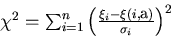 |
(3) |
where  is i-th measured coordinate,
 is its error, and
 is the expected i-th coordinate, when the
helix parameter vector is
is the expected i-th coordinate, when the
helix parameter vector is  .
What we need is the helix parameter vector which zeros
the first derivative of :
.
What we need is the helix parameter vector which zeros
the first derivative of :
| 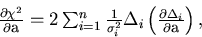 |
(4) |
where we have defined the i-th residual  by
by
| 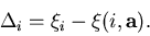 |
(5) |
This can be numerically found by iteratively from the following
equation (multi-dimensional Newton's method):
| 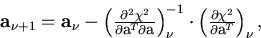 |
(6) |
where the left-hand side is the  -th estimate of the
helix parameter vector based on the knowledge on the
right-hand side of its
-th estimate of the
helix parameter vector based on the knowledge on the
right-hand side of its
 -th estimate together with the first and the second derivatives of
the thereat.
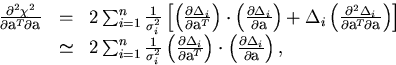
The second derivative is given by
-th estimate together with the first and the second derivatives of
the thereat.
The second derivative is given by
|  |
(7) |
where in the last line
we have deliberately left out the second derivatives of 's
in order to make positive definite the second derivative matrix of
![[*]](foot_motif.gif) .
When the initial estimate of the parameter vector
.
When the initial estimate of the parameter vector  is
a good approximation, the parameter vector converges rapidly after a few
times of iterations.
Nevertheless, it is usually recommended to multiply the diagonal elements of the
second derivative matrix by some constant which is greater than unity
and try again, when
the increased for the new estimate of the parameter vector.
This prescription renders the parameter change vector along the opposite
gradient direction in such cases and stabilizes the fit.
is
a good approximation, the parameter vector converges rapidly after a few
times of iterations.
Nevertheless, it is usually recommended to multiply the diagonal elements of the
second derivative matrix by some constant which is greater than unity
and try again, when
the increased for the new estimate of the parameter vector.
This prescription renders the parameter change vector along the opposite
gradient direction in such cases and stabilizes the fit.
When the fit converges, the error matrix for the parameter vector is
obtained to be
| 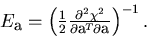 |
(8) |
It should be emphasized that
we have to carefully choose the helix parametrization so as to
numerically stabilize the fitting procedure: the helix parameters should
stay small and continuously change during the fit.
Notice that our parametrization allows a continuous transition from a
negative charge solution to a positive charge solution:
with other parameters stay the same.
Since this transition implies that the center of the helix jumps from a point
infinitely away on one side of the track to another infinitely away point
on the other side of the track, it changes the meaning of  discretely by
  .
.
Next: Change of Pivot
Up: General Discussions without Momentum
Previous: Helix Parametrization
Keisuke Fujii
12/4/1998