In order to estimate the actual sensitivity, we must take into account the helical trajectory in the solenoidal magnet of the detector. We assume a uniform field of 2 Tesla parallel to the z-axis. We detect the particle positions 1m downstream from the IP,i.e. z=+1m.
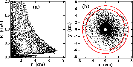
Figure 5:
Distributions of scattered particles at z=+1m, where
particles with r > 0.5cm are plotted. The particles are tracked in
helical trajectories in a magnetic field of ![]() =2 tesla. (a) is for
a scatter plot on the plane of the energy(E) and the radial
distance(r), and (b) is for a plot on the plane of x and y,
where two concentric circles of 6 and 7cm radii are also shown just
for an eye guide.
=2 tesla. (a) is for
a scatter plot on the plane of the energy(E) and the radial
distance(r), and (b) is for a plot on the plane of x and y,
where two concentric circles of 6 and 7cm radii are also shown just
for an eye guide.
Figures 5(a) and (b) show the radial and azimuthal
angular distributions of the particles, respectively. There is a
clear maximum radial boundary as a function of the energy in
Fig.5(a), as expected from the Eq.14.
Outside of the boundary only a relatively small number of the
particles can be seen, which have inherent angles larger than the
beam-beam deflection angle. We can also see another dense region at
r<1 cm corresponding to the opposite-charge particles(![]() ), as
described in the previous section. The most interesting particles
are distributed at the maximum radial distance of around r=7cm.
Since they have almost the same magnitude as the energy, as clearly
shown in Fig.5(a), their original azimuthal
distribution should be preserved even after they flowed in the
magnetic field. Actually, this expectation is realized as in
Fig.5(b), where we can clearly see two sides of the
depleted region, especially for 6<r<7cm. The two sides are sitting
on a line rotated counter-clockwise by
), as
described in the previous section. The most interesting particles
are distributed at the maximum radial distance of around r=7cm.
Since they have almost the same magnitude as the energy, as clearly
shown in Fig.5(a), their original azimuthal
distribution should be preserved even after they flowed in the
magnetic field. Actually, this expectation is realized as in
Fig.5(b), where we can clearly see two sides of the
depleted region, especially for 6<r<7cm. The two sides are sitting
on a line rotated counter-clockwise by ![]() 70
70![]() , which
corresponds to the horizontal direction.
, which
corresponds to the horizontal direction.