Track Fitting under the Influence of Multiple Scattering

When the track is affected by multiple scattering during its coordinate measurements the error matrix (E₀ in Eq.3.2.15) should take that into account. To see how to implement multiple scattering, let us start with the modification of the track equation (Eq.3.2.7):

$$\begin{array} {lll} \nonumber \frac{d {\bf a}}{dy} = - T \cdot {\bf a},\end{array}$$

where we have set (x₀,y₀) = (0,0) and $y \equiv \Delta y_0$.Multiple scattering modifies $\eta$ by

$$\begin{array} {lll} d\eta \equiv d\phi_0 = \left( \frac{d\phi}{dy} \right) ~ dy\end{array}$$ (58)

which necessitates the modification of the track equation to

$$\begin{array} {lll} \frac{d {\bf a}}{dy} = - T \cdot {\bf a} + \pmatrix{ 0 \cr \frac{d\phi}{dy} \cr 0 }.\end{array}$$ (59)

This means

$$\begin{array} {lll} \left\{ \begin{array} {lllllll} \xi(y) ... ... & = & \kappa_0 , & ~ & ~ & ~ & ~ \end{array}\right.\end{array}$$ (60)

where the suffix attached to the track track parameters remines us that they are the track parameters at the starting point before any multiple scattering. In the pivot convention taken here (x₀,y₀) = (0,0), $\xi(y)$ is the x-location of the track. Therefore, the probability of observing (n+1) hit points, $(x_i,y_i); i=0,1,\cdots,n$ and $y_0=0, \cdots, y_n = L$, is

$$\begin{array} {lll} P_M({\bf x};\phi;{\bf a}_0) = N ~ \exp... ...;\phi;{\bf a}_0)} {\sigma_{x_i} }\right)^2 \right],\end{array}$$ (61)

where N is a normalization factor and ${\bf x} \equiv (x_0,\cdots,x_n)^T$.We must, however, take into account the probability of obtaining the multiple scattering $\phi(y)$:

$$\begin{array} {lll} P_{MS}(\phi;{\bf a}_0) & = & N' \exp ... ...c{1}{K} \left(\frac{d\phi}{dy}\right)^2 dy \right],\end{array}$$ (62)

where use has been made of Eq.3.2.11. Since we do not know $\phi(y)$, we should integrate the probability over $\phi(y)$: 

$$\begin{array} {lll} \overline{P}({\bf x};{\bf a}_0) & = &... ...;\phi;{\bf a}_0)} {\sigma_{x_i} }\right)^2 \right],\end{array}$$ (63)

which now gives the probability of observing ${\bf x} = (x_0,\cdots,x_n)$ when the track has the track parameter ${\bf a}_0$ at y=0.

Now, we fit the (n+1) hits to our track model (Eq.3.1.1) by minimizing

$$\begin{array} {lll} \chi^2 = \sum_{i=0}^n \left(\frac{x_i-x(y_i,{\bf a})}{\sigma_{x_i}}\right)^2\end{array}$$ (64)

where $x(y,{\bf a})$ is given by Eq.3.1.1 with x₀=0. Since this problem is linear, we can easily obtain  

$$\begin{array} {lll} {\bf a} = E_M \cdot \sum_{i=0}^n \frac{... ...-y_i \cr \frac{y_i^2}{2\alpha} \end{array} \right)\end{array}$$ (65)

with

$$\begin{array} {lll} E_M^{-1} = \left( \begin{array} {rrr} ... ...\frac{y_i^4}{\sigma_{x_i}^2} \end{array} \right) ,\end{array}$$ (66)

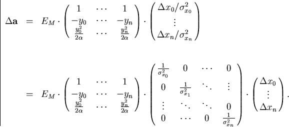
where E_M^-1 is the inverse of the error matrix due to corrdinate measurement errors, for which only the upper triangle is explicitly shown. Of course, the true error matrix is subsect to the correction for multiple scattering. Let us now derive the true error matrix below. We first note that the displacement of ${\bf x}$ induces the displacement of ${\bf a}$ through Eq.3.2.34:  

$$\begin{array} {lll} \Delta {\bf a} & = & E_M \cdot \pmatr... ...t \pmatrix{ \Delta x_0 \cr \vdots \cr \Delta x_n }. \end{array}$$ (67)

Defining A and $E_{\bf x}$ by  

$$\begin{array} {lll} A \equiv \pmatrix{ 1 & \cdots & 1 \cr ... ... \ddots & 0 \cr 0 & \cdots & 0 & \sigma_{x_n}^2 },\end{array}$$ (68)

we can rewrite Eq.3.2.36 as  

$$\begin{array} {lll} \Delta {\bf a} = E_M \cdot A \cdot E_{\bf x}^{-1} \cdot \Delta {\bf x}.\end{array}$$ (69)

This equation implies the full error matrix including multiple scattering to be given by  

$$\begin{array} {lll} \left< \Delta {\bf a} \cdot \Delta {\bf... ...right\gt \cdot E_{\bf x}^{-1} \cdot A^T \cdot E_M .\end{array}$$ (70)

Notice that in the absence of multiple scattering, we have

$$\begin{array} {lll} \nonumber \left< \Delta {\bf x} \cdot \Delta {\bf x}^T \right\gt = E_{\bf x}\end{array}$$

and, therefore,

$$\begin{array} {lll} \nonumber \left< \Delta {\bf a} \cdot \... ...ot E_M \cr & = & E_M \cdot E_M^{-1} \cdot E_M = E_M\end{array}$$

as it should be, where in the last line, we have used

$$\begin{array} {lll} \left( A \cdot E_{\bf x}^{-1} \cdot A^T \right) = E_M^{-1}\end{array}$$ (71)

which can be readily verified.

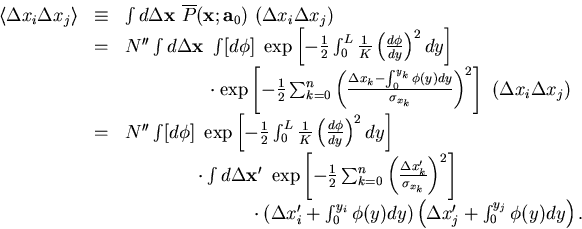
Our problem is now reduces to how to evaluate $\left< \Delta {\bf x} \cdot \Delta {\bf x}^T \right\gt$ when the multiple scattering correlates, for instance, $\Delta x_i$ to $\Delta x_j$.In order to calculate the correlation matrix, we first note that

$$\begin{array} {lll} \begin{array} {llllllc} \Delta x_i & = ... ...rajectory} & ~ & \int_0^{y_i} \phi(y) dy\end{array}\end{array}$$ (72)

Substituting this in Eq.3.2.32, we obtain the following formula for the probability of getting the measured points ${\bf x} = (x_0,x_1,\cdots,x_n)^T$for a track whose track parameter vector at y=y₀ is ${\bf a}_0$:

$$\begin{array} {lll} \overline{P}({\bf x};{\bf a}_0) & = & ... ...y_i} \phi(y) dy} {\sigma_{x_i}} \right)^2 \right],\end{array}$$ (73)

which leads us to

$$\begin{array} {lll} \nonumber \left<\Delta x_i \Delta x_j \... ...left(\Delta x'_j + \int_0^{y_j} \phi(y) dy \right) .\end{array}$$

The $\Delta {\bf x'}$ integral is readily performed to yield  

$$\begin{array} {lll} \left<\Delta x_i \Delta x_j \right\gt ... ... dy \right) \left(\int_0^{y_j} \phi(y) dy \right) .\end{array}$$ (74)

The second term, which was induced by multiple scattering, has a familiar path integral form in field theories. After some straightforward manipulations such as to divide the path into small segments and to replace integrals by summentions and differentiations by differences, we arrive at  

$$\begin{array} {lll} \mbox{the 2nd term} \equiv B_{ij} = \frac{K}{2} y_i^2 ( y_j - y_i/3 )\end{array}$$ (75)

for $i \leq j$ which is enough since B is apparently symmetric. Combining Eqs.3.2.39, 3.2.46, and 3.2.47, we obtain the full error matrix as the sum of the part due to coordinate measurement errors E_M and the part due to the multiple scattering in the tracking volume E_MS:  

$$\begin{array} {lll} E \equiv \left< \Delta {\bf a} \cdot \Delta {\bf a}^T \right\gt = E_M + E_{MS}\end{array}$$ (76)

with  

$$\begin{array} {lll} E_{MS} = E_M \cdot A \cdot E_{\bf x}^{-... ... \cdot B \cdot E_{\bf x}^{-1} \cdot A^T \cdot E_M .\end{array}$$ (77)

The calculation of E_MS is tedious but doable. We will, however, restrict ourselves to the case where the (n+1) samples are equally spaced in y and measured with an equal accuracy $\sigma_x$.We fill further assume that n is large, since the final expression otherwise becomes too complicated to show here. The large n limit then gives

$$\begin{array} {lll} E_M & \simeq & \sigma_x^2 \pmatrix{... ...^3}\cr ~ & ~ & \frac{180 \cdot (2\alpha)^2}{nL^4} }\end{array}$$ (78)

and

$$\begin{array} {lll} E_{MS} & \simeq & K \left( \begin{arr... ...& \frac{5 (2\alpha)^2}{14 L} \end{array} \right) ,\end{array}$$ (79)

which, for instance, result in

$$\begin{array} {lll} \nonumber \left(\sigma_\kappa^{MS}\righ... ...ght)_{33} = \frac{10}{7} \cdot \frac{K\alpha^2}{L}.\end{array}$$

The error on $\kappa \equiv Q/P_T$ due to multiple scattering is thus obtained to be

$$\begin{array} {lll} \nonumber \left(\sigma_\kappa^{MS}\righ... ... \left(\frac{C}{P_T\beta}\right)^2 \frac{X}{X_0}, \end{array}$$

where use has been made of Eq.3.2.11 and

$$\begin{array} {lll} \nonumber P_T^2 & = & P^2/(1+\tan^2\lambda) \cr X & \equiv & (1+\tan^2\lambda)^{1/2} L.\end{array}$$

The X is the material thickness through which the track passes. To see the dependence on the magnetic field explicitly, we introduce a new constant $\alpha'$ defined by

$$\begin{array} {lll} \nonumber \alpha' \equiv \alpha \cdot B.\end{array}$$

When we assume $\beta = 1$ and |Q|=1 (unit charge), we finally get a familiar result:  

$$\begin{array} {lll} \sigma_\kappa^{MS}/ \kappa = \frac{\a... ...C}{LB} \sqrt{\frac{10}{7}\left(\frac{X}{X_0}\right)}\end{array}$$ (80)

with

$$\begin{array} {lll} \left\{ \begin{array} {lll} \alpha' &... ... & \mbox{magnetic field (T)} \end{array} \right. .\end{array}$$ (81)