Next: Performance of fit by ks
Up: Performance of geometrical constraint
Previous: Performance of geometrical constraint
Here we consider to find the common vertex consisting of N
charged tracks. Let their track parameters and error matrixes are
 and
and  .
Track parameter consists of 5 elements: dri,
.
Track parameter consists of 5 elements: dri,
 ,
,
 ,
dzi, and
,
dzi, and
 .
In the geometrical constraint fit, are fitted by vertex coordinate,
.
In the geometrical constraint fit, are fitted by vertex coordinate,  ,
and
fitted helix parameter,
,
and
fitted helix parameter,  .
consists of three elements:
.
consists of three elements:
 ,
,
 ,
and
,
and
 .
Parameters corresponding to driand dzi are zero as we constraint
to go through the
common vertex point .
.
Parameters corresponding to driand dzi are zero as we constraint
to go through the
common vertex point .
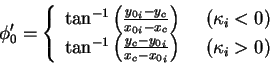
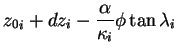
A helix, in terms of a, is expressed as
where, (
x0i, y0i, z0i) is the pivot and
 is a deflection angle relative to the pivot.
The same helix can be expressed, in terms of  as,
as,
Using b, the
center of the circle is given by
 |
(7) |
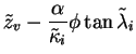
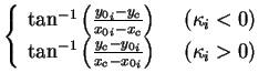
Therefore, the deflection angle at the pivot of input helix is given by
 |
(8) |
Note that  is a deflection angle for the input helix estimated from the fitting parameter
b.
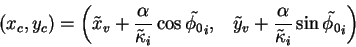
The expected position of the helix at the pivot of the input helix is
is a deflection angle for the input helix estimated from the fitting parameter
b.
The expected position of the helix at the pivot of the input helix is
| x' |
= |
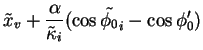 |
(9) |
| y' |
= |
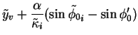 |
(10) |
| z' |
= |
 |
(11) |
Using these formula, the helix parameter is expressed as follows by
the fitting parameter b:
| dr' |
= |
![$\displaystyle \left[ x' - {x_0}_i \right]\cos\phi_0'
+ \left[ y' - {y_0}_i \right]\sin\phi_0'$](img29.gif) |
(12) |
 |
= |
 |
(13) |
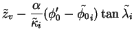
 |
= |
 |
(14) |
| dz' |
= |
z' - z0i |
(15) |
 |
= |
 |
(16) |
12pt
What we do in the geometrical constraint is to minimize  defined as
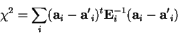 |
(17) |
where
 is the helix parameter of i-th track derived from
the fitting parameter b:
dr', ,
is the helix parameter of i-th track derived from
the fitting parameter b:
dr', ,
 ,
dz', and
,
dz', and
 .
is a function of b, and we find the parameter b
by using the Newtonian method.
.
is a function of b, and we find the parameter b
by using the Newtonian method.
The principle of the Newtonian method is as follows.
can be expanded with respect to b as,
 |
(18) |
where
 ,
,
 is
the parameter in the current iteration loop and
is
the parameter in the current iteration loop and
 is the parameter for
the next iteration.
If we use the terms up to second order,
can be expressed as
is the parameter for
the next iteration.
If we use the terms up to second order,
can be expressed as
![\begin{displaymath}\chi^2 = {1\over 2} {\partial^2\chi^2 \over \partial {\bf b}^...
...-1}
{\partial \chi^2 \over \partial {\bf b}} \right] + Const.
\end{displaymath}](img44.gif) |
(19) |
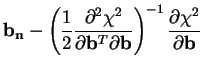
and
 to minimize
is given by
to minimize
is given by
 |
(20) |
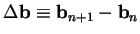
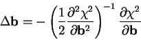
Namely the parameter for next iteration is given by
Note that the second derivative in Eq. 22,
 represents the local curvature of the
surface of b coordinate system. If we use the exact form of the
second derivative in the minimization, it becomes sensitive to the local
property of the surface and the fitting process becomes to slow or divergent.
To avoid this problem, we multiply the diagonal part of the matrix
by a factor
represents the local curvature of the
surface of b coordinate system. If we use the exact form of the
second derivative in the minimization, it becomes sensitive to the local
property of the surface and the fitting process becomes to slow or divergent.
To avoid this problem, we multiply the diagonal part of the matrix
by a factor
 .
.
In the class JSFVirtualFit, from which JSFGeoCFit is derived,
the initial value of  is 10-12,
but is is multiplied by 100 or divided by 100 depending on the change of .
The fit converged if the change of
during the minimization loop
becomes less than 10-6. The loop is abandoned if
the number of loop exceeds 50 or
becomes larger than 1060.
is 10-12,
but is is multiplied by 100 or divided by 100 depending on the change of .
The fit converged if the change of
during the minimization loop
becomes less than 10-6. The loop is abandoned if
the number of loop exceeds 50 or
becomes larger than 1060.
The derivatives and the second derivatives of
with respect to b is given
in the appendix 1.
Next: Performance of fit by ks
Up: Performance of geometrical constraint
Previous: Performance of geometrical constraint
akiya miyamoto
2000-02-28
![$\displaystyle {x_0}_i + d\rho_i\cos{\phi_0}_i + {\alpha\over\kappa_i}
\left[\cos{\phi_0}_i - \cos(\phi+{\phi_0}_i)\right]$](img13.gif)
![$\displaystyle {y_0}_i + d\rho_i\sin{\phi_0}_i + {\alpha\over\kappa_i}
\left[\sin{\phi_0}_i - \sin(\phi+{\phi_0}_i)\right]$](img15.gif)
![$\displaystyle \tilde{x}_v + {\alpha\over\tilde{\kappa}_i}
\left[\cos\tilde{\phi_0}_i - \cos(\phi+\tilde{\phi_0}_i)\right]$](img20.gif)
![$\displaystyle \tilde{y}_v + {\alpha\over\tilde{\kappa}_i}
\left[\sin\tilde{\phi_0}_i - \sin(\phi+\tilde{\phi_0}_i)\right]$](img21.gif)